Random Forest with Smile & Tablesaw
While linear regression analysis (introduced in the Moneyball tutorial) is widely used and works well for a variety of problems, tree-based models provide excellent results and be applied to datasets with both numerical and categorical features, without making any assumption of linearity. In addition, tree based methods can be used effectively for regression and classification tasks.
This tutorial is based on Chapter 8 (Tree Based Methods) of the widely used and freely available textbook An Introduction to Statistical Learning, Second Edition.
Basic Decision Trees
The basic idea of a decision tree is simple: use a defined, algorithmic approach to partition the feature space of a dataset into regions in order to make a prediction. For a regression task, this prediction is simply the mean of the response variable for all training observations in the region. In any decision tree, every datapoint that falls within the same region receives the same prediction.
The following figure illistrates a two-dimensional feature space that has been partitioned according to a greedy algorithm that minimizes the residual sum of squares.
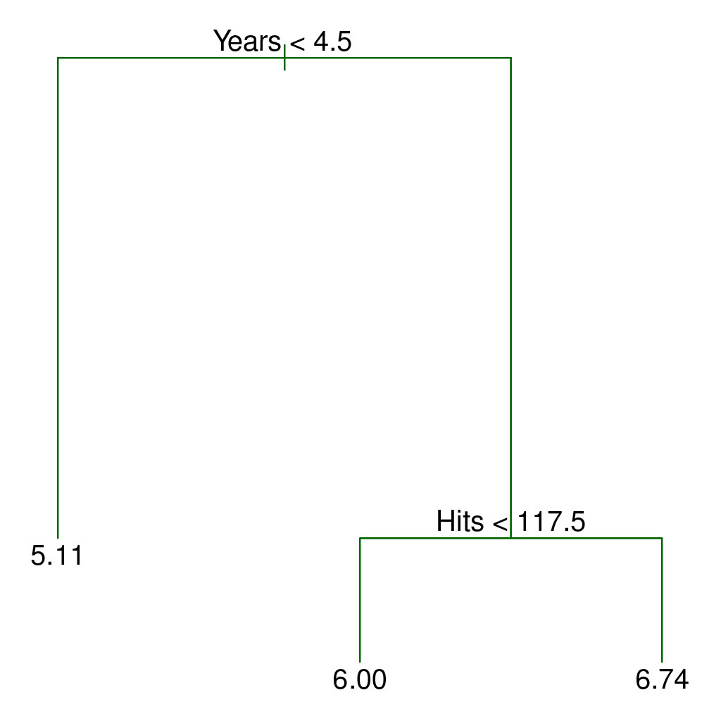
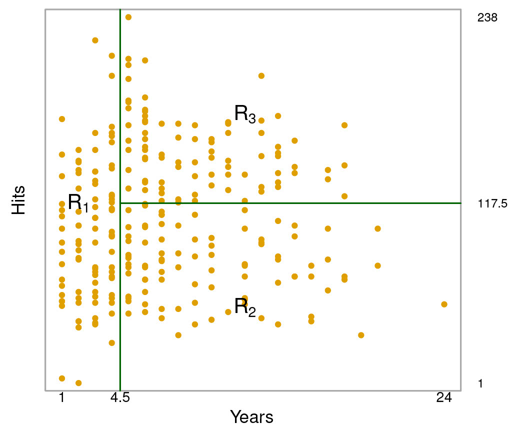
Credit: An Introduction to Statistical Learning, Second Edition Figures 8.1 and 8.2
As you can see, the feature space is split into three regions, and three predictions are possible: 5.00, 6.00, and 6.74.
While decision trees are easily interpretable, especially when looking at the visual of the tree, basic decision trees like this one are generally less accurate than other regression/classification approaches. More advanced tree-based methods, however, not only compete with other approaches, but often provide exceptional performance.
Random Forest
Random Forest is an ensemble method that builds on basic decision trees to form a model that is the composition of a large number of individual decision trees. In a Random Forest model, n decision trees are grown independently, with each tree considering only a subset of of predictors m, using only a subset of the training data. Becuase the majority of the predictors are not considered in each individual tree, the predicitons of each individual tree are decorrelated and therefore the average decision of all the trees in the model will have lower variance and be of greater predictive value. The greedy algorithm used to construct decision trees is heavily influenced by strong predictors, so by excluding a number of predictors when each tree in the Random Forest is grown, the model can explore the predictive value of other features that previously may have been largely ignored.
Implementing Random Forest for the Heart dataset using Tablesaw + Smile
The Heart dataset contains 13 qualitative and quantitative predictors for 303 patients who sought medical attention due to chest pain. The response represents a binary classification scenario as we want to predict which patients have heart disease and which do not. You can download the dataset here.
As usual, you will need to add the smile, tablesaw-core, and tablesaw-jsplot dependencies. (Described in Moneyball Tutorial)
First, load and clean the data. Qualitative features must be represented as integers to build the model.
Table data = Table.read().csv("Heart.csv");

//encode qualitative features as integers to prepare for Smile model.
data.replaceColumn("AHD", data.stringColumn("AHD").asDoubleColumn().asIntColumn());
data.replaceColumn("Thal", data.stringColumn("Thal").asDoubleColumn().asIntColumn());
data.replaceColumn("ChestPain", data.stringColumn("ChestPain").asDoubleColumn());

//Remove the index column, as it is not a feature
data.removeColumns("C0");

//Remove rows with missing values
data = data.dropRowsWithMissingValues();

//print out cleaned dataset for inspection
System.out.println(data.printAll());
Next, segment your dataset into two distinct tables. Rows are randomly assigned tables by default using the .sampleSplit() function.
//Split the data 70% test, 30% train
Table[] splitData = data.sampleSplit(0.7);
Table dataTrain = splitData[0];
Table dataTest = splitData[1];
Now build an initial RandomForest model using the training dataset and sensible parameter values. m, the number of features to be considered for each tree, is set to the square root of the number of features. n, or ntrees, is set to 50, a reasonmable starting point that will run quickly. d, or maxDepth, is the maximum depth of any individual decision tree, and is set to another reasonable value, 7. maxNodes is set to 100 and represents the most number of terminal decision making nodes a tree can have. All of these values are considered Hyperparameters and should be refined by the user to improve the accuracy of the model.
Note: Smile contains two RandomForest classes, one for classification tasks and one for regression tasks. Make sure you import the correct class for your problem context, in this case smile.classification.RandomForest
//initial model with sensible parameters
RandomForest RFModel1 = smile.classification.RandomForest.fit(
     Formula.lhs("AHD"),
     dataTrain.smile().toDataFrame(),
     50, //n
     (int) Math.sqrt((double) (dataTrain.columnCount() - 1)), //m = sqrt(p)
     SplitRule.GINI,
     7, //d
     100, //maxNodes
     1,
     1
);
View the first decision tree generated by the model.
System.out.println(RFModel1.trees()[0]);
Predict the response of the test dataset using your model and assess model accuracy.
//predict the response of test dataset with RFModel1
int[] predictions = RFModel1.predict(dataTest.smile().toDataFrame());

//evaluate % classification accuracy for RFModel1
double accuracy1 = Accuracy.of(dataTest.intColumn("AHD").asIntArray(), predictions);
System.out.println(accuracy1);
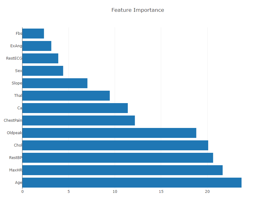
Generate and plot feature importance. According to the Smile documentation, the built in .importance() function calculates variable importance as the sum decrease in the Gini impurity criterion across all node splits on that variable, averaged across all trees in the Random Forest. In other words, the more that impurity declines when a node is split on a variable, the more important it is to the predictive power of a model.
//measure variable importance (mean decrease Gini Index)
double[] RFModel1_Importance = RFModel1.importance();
System.out.println(Arrays.toString(RFModel1_Importance));

//plot variable importance with tablesaw
Table varImportance = Table.create("featureImportance");
List<String> featureNames = dataTrain.columnNames();
featureNames.remove(13); //remove response
varImportance.addColumns(DoubleColumn.create("featureImportance", RFModel1_Importance), StringColumn.create("Feature",  featureNames));
varImportance = varImportance.sortDescendingOn("featureImportance");
Plot.show(HorizontalBarPlot.create("Feature Importance", varImportance, "Feature", "featureImportance"));
As you can see, features Fbs and ExAng have the lowest importance in the model, while Age, MaxHR, RestBP, and Chol are all of high importance.
Another (lesser) concern when selecting features to include in the model is having two features that are highly correlated with one another. At best, including all of such features is redundant, at worst, it could negatively impact model performance.
Spearman’s correlation metric provides a measure of feature correlation and can be generated automatically with Tablesaw. (-1 represents an extreme negative correlation, +1 represents an extreme positive correlation)
Generate a matrix of Spearman’s correlation metrics between all features.
        //construct correlation matrix
        Table corr = Table.create("Spearman's Correlation Matrix");
        corr.addColumns(StringColumn.create("Feature"));
        for(String name: dataTest.columnNames().subList(0,12))
        {
            corr.addColumns(DoubleColumn.create(name));
        }
        for(int i = 0; i < 12; i++)
        {
            for(int j = 0; j < 12; j++)
            {
                corr.doubleColumn(i+1).append(dataTrain.numericColumns(i).get(0).asDoubleColumn().spearmans(dataTrain.numericColumns(j).get(0).asDoubleColumn()));
            }
        }
        corr.stringColumn("Feature").addAll(dataTrain.columnNames().subList(0,12));

        for(Object ea: corr.columnsOfType(ColumnType.DOUBLE))
        {
            ((NumberColumn) ea).setPrintFormatter(NumberColumnFormatter.fixedWithGrouping(2));
        }

        System.out.println(corr.printAll());
Output:
>                                                         Spearman's Correlation Matrix
  Feature   |   Age   |   Sex   |  ChestPain  |  RestBP  |  Chol   |   Fbs   |  RestECG  |  MaxHR  |  ExAng  |  Oldpeak  |  Slope  |   Ca    |
----------------------------------------------------------------------------------------------------------------------------------------------
       Age  |   1.00  |  -0.08  |      -0.18  |    0.34  |   0.14  |   0.08  |     0.16  |  -0.41  |   0.10  |     0.23  |   0.16  |   0.34  |
       Sex  |  -0.08  |   1.00  |      -0.11  |   -0.06  |  -0.13  |   0.04  |     0.01  |  -0.05  |   0.10  |     0.13  |   0.03  |   0.13  |
 ChestPain  |  -0.18  |  -0.11  |       1.00  |   -0.15  |  -0.02  |   0.04  |    -0.11  |   0.29  |  -0.33  |    -0.33  |  -0.28  |  -0.20  |
    RestBP  |   0.34  |  -0.06  |      -0.15  |    1.00  |   0.11  |   0.12  |     0.15  |  -0.09  |   0.06  |     0.20  |   0.10  |   0.07  |
      Chol  |   0.14  |  -0.13  |      -0.02  |    0.11  |   1.00  |   0.03  |     0.17  |  -0.07  |   0.09  |     0.03  |  -0.01  |   0.07  |
       Fbs  |   0.08  |   0.04  |       0.04  |    0.12  |   0.03  |   1.00  |     0.06  |  -0.03  |   0.05  |     0.01  |  -0.00  |   0.17  |
   RestECG  |   0.16  |   0.01  |      -0.11  |    0.15  |   0.17  |   0.06  |     1.00  |  -0.07  |   0.03  |     0.11  |   0.16  |   0.13  |
     MaxHR  |  -0.41  |  -0.05  |       0.29  |   -0.09  |  -0.07  |  -0.03  |    -0.07  |   1.00  |  -0.46  |    -0.41  |  -0.40  |  -0.26  |
     ExAng  |   0.10  |   0.10  |      -0.33  |    0.06  |   0.09  |   0.05  |     0.03  |  -0.46  |   1.00  |     0.29  |   0.27  |   0.22  |
   Oldpeak  |   0.23  |   0.13  |      -0.33  |    0.20  |   0.03  |   0.01  |     0.11  |  -0.41  |   0.29  |     1.00  |   0.60  |   0.30  |
     Slope  |   0.16  |   0.03  |      -0.28  |    0.10  |  -0.01  |  -0.00  |     0.16  |  -0.40  |   0.27  |     0.60  |   1.00  |   0.10  |
        Ca  |   0.34  |   0.13  |      -0.20  |    0.07  |   0.07  |   0.17  |     0.13  |  -0.26  |   0.22  |     0.30  |   0.10  |   1.00  |
Features Slope and Oldpeak have a moderate positive correlation of 0.6, the largest in the table. I will opt to leave both features in the dataset as their correlation is likely not strong enough to distort the model.
Based on the feature importance plot, I will cut Fbs from the feature space.
//cut variables
dataTest.removeColumns("Fbs");
dataTrain.removeColumns("Fbs");
Now, we can generate a second model using the selected features.
RandomForest RFModel2 = smile.classification.RandomForest.fit(
     Formula.lhs("AHD"),
     dataTrain.smile().toDataFrame(),
     50, //n
     (int) Math.sqrt((double) (dataTrain.columnCount() - 1)), //m = sqrt(p)
     SplitRule.GINI,
     7, //d
     100, //maxNodes
     1,
     1
);
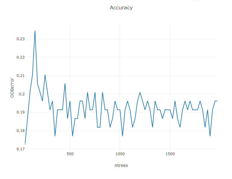
Now, lets determine an appropriate number of trees to grow in the model. A good rule of thumb is to select a number of trees that is the least number required to achieve minimum out-of-bag error when building the model. To determine this, we can graph OOBError vs ntrees.
//tuning ntrees
Table AccuracyvTrees = Table.create("OOB-Error vs nTrees");
AccuracyvTrees.addColumns(DoubleColumn.create("OOBerror"), DoubleColumn.create("ntrees"));

 for(int j = 50; j < 2000; j = j+25)
       {
           RandomForest model = smile.classification.RandomForest.fit(
           Formula.lhs("AHD"),
           dataTrain.smile().toDataFrame(),
           j,
           (int) Math.sqrt((double) (dataTrain.columnCount() - 1)), //root p
           SplitRule.GINI,
           7,
           100,
           1,
           1
            );

            double err = model.error();
            AccuracyvTrees.doubleColumn(0).append(err);
            AccuracyvTrees.doubleColumn(1).append(j);
        }

Plot.show(LinePlot.create("Accuracy", AccuracyvTrees, "ntrees", "OOBerror"));
The Out-of-bounds error appears to settle down after ~1,000 trees. (your plot may look slightly different due to randomness in splitting the dataset and in the model algorithm). To be conservative, we can select 1,200 trees as the parameter of our final model.
We can now build and assess our final model using our new value for ntrees.
//model with graph-selected number of trees
RandomForest RFModelBest = smile.classification.RandomForest.fit(
    Formula.lhs("AHD"),
    dataTrain.smile().toDataFrame(),
    1200,
    (int) Math.sqrt((double) (dataTrain.columnCount() - 1)), //root p
    SplitRule.GINI,
    7,
    100,
    1,
    1
    );

int[] predictionsBest = RFModelBest.predict(dataTest.smile().toDataFrame());
double accuracyBest = Accuracy.of(dataTest.intColumn("AHD").asIntArray(), predictionsBest);
System.out.println(accuracyBest);

> 0.8333333333333334
The classification accuracy of my final model was ~83%. So, using a relatively small dataset, the Random Forest algorithm is able to correctly predict whether or not a patient has heart disease ~83% of the time.
Recap
We used Tablesaw to clean the Heart dataset and prepare it for the Random Forest algorithm. We generated a sensible starting model and plotted its Gini Index importance and Spearman’s correlation matrix to identify features to cut from the model. We then used out-of-bounds error to identify a large enough number of trees to include in the model to achieve maximum accuracy with limited computation time.
Extensions
While the classic method of splitting the dataset 70% test, 30% train works reasonably well, for smaller datasets your model performance metrics can experience some variation due to having a training dataset of limited size. For such datasets, validation procedures such as n-fold cross validation and leave one out cross validation may be more appropriate. Smile includes built-in functions to perform cross validation.
In addition, in this example we only tuned the ntrees hyperparameter; adjustments to mtry, maxDepth, maxNodes, and nodeSize could be considered as well.