Moneyball: Linear Regression with Smile & Tablesaw
Linear regression analysis has been called the “Hello World” of machine learning, because it’s widely used and easy to understand. It’s also very powerful. We’ll walk through the modeling process here using Smile and Tablesaw. Smile is a fantastic Java machine learning library and Tablesaw is data wrangling library like pandas.
One of the best known applications of regression comes from the book Moneyball, which describes the innovative use of data science at the Oakland A’s baseball team. My analysis is based on a lecture given in the EdX course: MITx: 15.071x The Analytics Edge. If you’re new to data analytics, I would strongly recommend this course.
Moneyball is a great example of how to apply data science to solve a business problem. For the A’s, the business problem was “How do we make the playoffs?” They break that problem down into simpler problems that can be solved with data. Their approach is summarized in the diagram below:
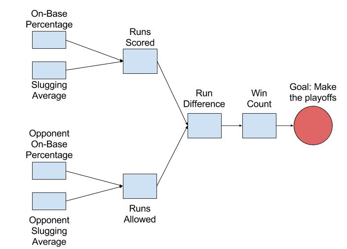
In baseball, you make the playoffs by winning more games than your rivals, but you can’t control the number of games your rivals win. How should you proceed? The A’s needed to find controllable variables that affected their likelihood of making the playoffs.
Specifically, they wanted to know how to spend their salary dollars to produce the most wins. Statistics like “Batting Average” are available for individual players so if you knew Batting Average had the greatest impact, you can trade for players with high batting averages, and thus improve your odds of success.
To do regression modeling in Tablesaw, we’ll first need to import Smile:
//Gradle
// https://mvnrepository.com/artifact/com.github.haifengl/smile-core
    implementation group: 'com.github.haifengl', name: 'smile-core', version: '2.0.0'
//Maven
<dependency>
  <groupId>com.github.haifengl</groupId>
  <artifactId>smile-core</artifactId>
  <version>2.0.0</version>
</dependency>
(you will also need tablesaw-core and tablesaw-jsplot)
To connect player stats to making the playoffs, they systematically decomposed their high-level goal. They started by asking how many wins they’d need to make the playoffs. They decided that 95 wins would give them a strong chance. Here’s how we might check that assumption in Tablesaw. (Download CSV here)
// Get the data
Table baseball = Table.read().csv("data/baseball.csv");

// filter the data to start at the 2002 season when the A's model was made
Table moneyball = baseball.where(baseball.intColumn("year").isLessThan(2002));
We can check the assumption visually by plotting wins per year in a way that separates the teams who make the playoffs from those who don’t. This code produces the chart below:
NumericColumn wins = moneyball.nCol("W");
NumericColumn year = moneyball.nCol("Year");
Column playoffs = moneyball.column("Playoffs");
Figure winsByYear = ScatterPlot.create("Regular season wins by year", moneyball, "W", "year", "playoffs");
Plot.show(winsByYear);

Teams that made the playoffs are shown as yellow points. If you draw a vertical line at 95 wins, you can see that it’s likely a team that wins more than 95 games will make the playoffs. So far so good.
Aside: Visualization
The plots in this post were produced using Tablesaw’s new plotting capabilities. We’ve created a wrapper for much of the amazing Plot.ly open-source JavaScript plotting library. The plots can be used interactively in an IDE or delivered from a server. This is an area of active development. Support for advanced features continue to be added.
At this point we continue developing our model, but for those interested, this next section shows how to use cross-tabs to quantify how teams with 95+ wins have faired in getting to the playoffs.
Aside: Cross Tabs
We can also use cross-tabulations (cross-tabs) to quantify the historical data. Cross-tabs calculate the number or percent of observations that fall into various groups. Here we’re interested in looking at the interaction between winning more than 95 games and making the playoffs. We start by making a boolean column for more than 95 wins, then create a cross tab between that column and the “playoffs” column.
// create a boolean column - 'true' means team won more than 95 games
BooleanColumn ninetyFivePlus = BooleanColumn.create("95+ Wins", wins.isGreaterThanOrEqualTo(95), wins.size());
moneyball.addColumns(ninetyFivePlus);

// calculate the column percents
Table xtab95 = moneyball.xTabColumnPercents("Playoffs", "95+ Wins");

for(Object ea: xtab95.columnsOfType(ColumnType.DOUBLE))
       {
           ((NumberColumn) ea).setPrintFormatter(NumberColumnFormatter.percent(1));
       }

>        Crosstab Column Proportions:
 [labels]  |  false   |   true   |  total   |
---------------------------------------------
      0.0  |   91.9%  |   18.2%  |   82.9%  |
      1.0  |    8.1%  |   81.8%  |   17.1%  |
           |  100.0%  |  100.0%  |  100.0%  |
As you can see from the table roughly 82% of teams who win 95 or more games also made the playoffs.
Unfortunately, you can’t directly control the number of games you win. We need to go deeper. At the next level, we hypothesize that the number of wins can be predicted by the number of Runs Scored during the season, combined with the number of Runs Allowed.
To check this assumption we compute Run Difference as Runs Scored - Runs Allowed:
NumberColumn RS = (NumberColumn) moneyball.numberColumn("RS");
NumberColumn RA = (NumberColumn) moneyball.numberColumn("RA");

NumberColumn runDifference = RS.subtract(RA).setName("RD");
moneyball.addColumns(runDifference);
Now lets see if Run Difference is correlated with Wins. We use a scatter plot again:
Figure runsVsWins = ScatterPlot.create("Run Difference x Wins", moneyball, "RD","W");
Plot.show(runsVsWins);
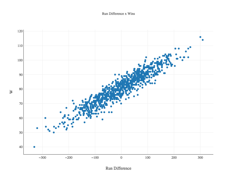
Our plot shows a strong linear relation between the two.
Modeling with OLS (Ordinary Least Squares) Regression
Let’s create our first predictive model using linear regression, with runDifference as the sole explanatory variable. Here we use Smile’s OLS (Ordinary Least Squares) regression model.
LinearModel winsModel = OLS.fit(Formula.lhs("W"), moneyball.selectColumns("RD", "W").smile().toDataFrame());
If we print our “winsModel”, it produces the output below:
Residuals:
	       Min	        1Q	    Median	        3Q	       Max
	  -14.2662	   -2.6511	    0.1282	    2.9365	   11.6570

Coefficients:
            		Estimate        Std. Error        t value        Pr(>|t|)
Intercept    		80.8814            0.1312       616.6747          0.0000 ***
Run Difference	     0.1058            0.0013        81.5536          0.0000 ***
---------------------------------------------------------------------
Significance codes:  0 '***' 0.001 '**' 0.01 '*' 0.05 '.' 0.1 ' ' 1

Residual standard error: 3.9391 on 900 degrees of freedom
Multiple R-squared: 0.8808,    Adjusted R-squared: 0.8807
F-statistic: 6650.9926 on 1 and 900 DF,  p-value: 0.000
Interpreting the model
If you’re new to regression, here are some take-aways from the output:
- The R-squared of .88 can be interpreted to mean that roughly 88% of the variance in Wins can be explained by the Run Difference variable. The rest is determined by some combination of other variables and pure chance.
- The estimate for the Intercept is the average wins independent of Run Difference. In baseball, we have a 162 game season so we expect this value to be about 81, as it is.
- The estimate for the RD variable of .1, suggests that an increase of 10 in Run Difference, should produce about 1 additional win over the course of the season.
Of course, this model is not simply descriptive. We can use it to make predictions. In the code below, we predict how many games we will win if we score 135 more runs than our opponents. To do this, we pass an array of doubles, one for each explanatory variable in our model, to the predict() method. In this case, there’s just one variable: run difference.
double[] runDifferential = {135};
double expectedWins = winsModel.predict(runDifferential);
  > 95.159733753496
We’d expect 95 wins when we outscore opponents by 135 runs.
Modeling Runs Scored
It’s time to go deeper again and see how we can model Runs Scored and Runs Allowed. The approach the A’s took was to model Runs Scored using team On-base percent (OBP) and team Slugging Average (SLG). In Tablesaw, we write:
LinearModel runsScored = OLS.fit(Formula.lhs("RS"), moneyball.selectColumns("RS", "OBP", "SLG").smile().toDataFrame());
Once again the first parameter takes a Tablesaw column containing the values we want to predict (Runs scored). The next two parameters take the explanatory variables OBP and SLG.
Linear Model:
Residuals:
           Min          1Q      Median          3Q         Max
      -70.8379    -17.1810     -1.0917     16.7812     90.0358

Coefficients:
            Estimate        Std. Error        t value        Pr(>|t|)
(Intercept)  -804.6271           18.9208       -42.5261          0.0000 ***
OBP          2737.7682           90.6846        30.1900          0.0000 ***
SLG          1584.9085           42.1556        37.5966          0.0000 ***
---------------------------------------------------------------------
Significance codes:  0 '***' 0.001 '**' 0.01 '*' 0.05 '.' 0.1 ' ' 1

Residual standard error: 24.7900 on 899 degrees of freedom
Multiple R-squared: 0.9296,    Adjusted R-squared: 0.9294
F-statistic: 5933.7256 on 2 and 899 DF,  p-value: 0.000
Again we have a model with excellent explanatory power with an R-squared of 92. Now we’ll check the model visually to see if it violates any assumptions. Our residuals should be normally distributed. We can use a histogram to verify:
Plot.show(Histogram.create("Runs Scored Residuals",runsScored.residuals()));
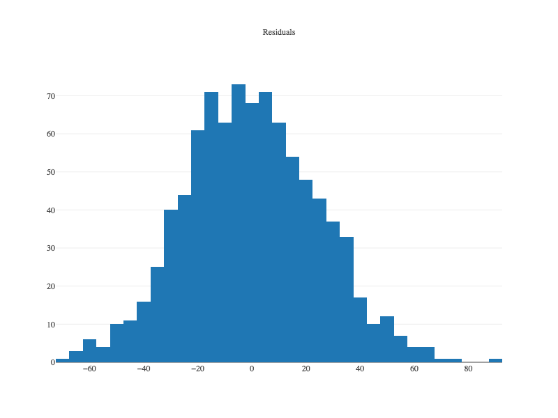
It looks great. It’s also important to plot the predicted (or “fitted”) values against the residuals. We want to see if the model fits some values better than others, which will influence whether we can trust its predictions or not. Ideally, we want to see a cloud of random dots around zero on the y axis.
Our Scatter class can create this plot directly from the model:
double[] fitted = runsScored.fittedValues();
double[] resids = runsScored.residuals();

Plot.show(ScatterPlot.create("Runs Scored from OBP and SLG", "Fitted", fitted, "Residuals", resids));
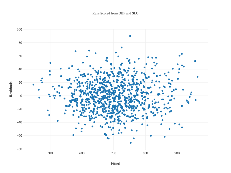
Again, the plot looks good.
Let’s review. We’ve created a model of baseball that predicts entry into the playoffs based on batting stats, with the influence of the variables as:
SLG & OBP -> Runs Scored -> Run Difference -> Regular Season Wins
Modeling Runs Allowed
Of course, we haven’t modeled the Runs Allowed side of Run Difference. We could use pitching and field stats to do this, but the A’s cleverly used the same two variables (SLG and OBP), but now looked at how their opponent’s performed against the A’s. We could do the same as these data are encoded in the dataset as OOBP and OSLG.
LinearModel runsAllowed = OLS.fit(Formula.lhs("RA"), moneyball.selectColumns("RA", "OOBP", "OSLG").dropRowsWithMissingValues().smile().toDataFrame());

> Linear Model:

Residuals:
	       Min	        1Q	    Median	        3Q	       Max
	  -82.3971	  -15.9782	    0.0166	   17.9137	   60.9553

Coefficients:
            Estimate        Std. Error        t value        Pr(>|t|)
Intercept  -837.3779           60.2554       -13.8971          0.0000 ***
OOBP	   2913.5995          291.9710         9.9791          0.0000 ***
OSLG	   1514.2860          175.4281         8.6319          0.0000 ***
---------------------------------------------------------------------
Significance codes:  0 '***' 0.001 '**' 0.01 '*' 0.05 '.' 0.1 ' ' 1

Residual standard error: 25.6739 on 87 degrees of freedom
Multiple R-squared: 0.9073,    Adjusted R-squared: 0.9052
F-statistic: 425.8225 on 2 and 87 DF,  p-value: 1.162e-45
This model also looks good, but you’d want to look at the plots again, and do other checking as well. Checking the predictive variables for collinearity is always good.
Finally, we can tie this all together and see how well wins is predicted when we consider both offensive and defensive stats.
LinearModel winsFinal = OLS.fit(Formula.lhs("W"), moneyball.selectColumns("W", "OOBP", "OBP", "OSLG", "SLG").dropRowsWithMissingValues().smile().toDataFrame());
The output isn’t shown, but we get an R squared of .89. Again this is quite good.
The A’s in 2001
For fun, I decided to see what the model predicts for the 2001 A’s. First, I got the independent variables for the A’s in that year.
StringColumn team2001 = moneyball.stringColumn("team");
NumberColumn year2001 = (NumberColumn) moneyball.numberColumn("year");

Table AsIn2001 = moneyball.selectColumns("year", "OOBP", "OBP", "OSLG", "SLG")
                .where(team2001.isEqualTo("OAK")
                .and(year2001.isEqualTo(2001)));

>                    baseball.csv
  Year   |  OOBP   |   OBP   |  OSLG  |   SLG   |
-------------------------------------------------
 2001.0  |  0.308  |  0.345  |  0.38  |  0.439  |
Now we get the prediction:
double[][] values = new double[][] 0.308;
double[] value = winsFinal.predict(values);
The model predicted that the 2001 A’s would win 102 games given their slugging and On-Base stats. They won 103.
Recap
We used regression to build predictive models, and visualizations to check our assumptions and validate our models.
The next step would involve predicting how the current team will perform using historical data, and find available talent who could increase the team’s average OBP or SLG numbers, or reduce the opponent values of the same stats. Taking it to that level requires individual player stats that aren’t in our dataset, so we’ll leave it here, but I hope this post has shown how Tablesaw and Smile work together to make regression analysis in Java easy and practical.